Advanced Encoding Once Again
In my previous article about how DXO achieves efficient compression, I mentioned that one of the ways it boosts compression efficiency is by introducing JPEG-XL, an advanced encoding format, to store the image data within the DNG.
The most famous DNG conversion software, Adobe DNG Converter, actually supports JPEG-XL encoding too. Although it hasn’t officially appeared in the UI yet, you can invoke this feature through command-line arguments, for example to achieve compression results similar to DXO:
EXE -lossy -jxl_effort 3 -jxl_distance 0.01 file.ARWThis combination of parameters produces a “Linear RAW” rather than a “Bayer RAW”, having already gone through demosaicing, linearisation and other processing. The file size may end up larger than the input RAW file. For instance, the losslessly compressed RAW file of a particular 33MP Sony a7C2 shot is 39.7MB, and after processing with Adobe DNG Converter it becomes 45.5MB, which clearly doesn’t quite meet our needs.
Through another parameter, -lossyMosaicJXL, you can output a Bayer RAW file compressed with JPEG-XL, but you can’t control the compression parameters. The actual settings used are JXL Effort 7, JXL Distance 0.2, and Decode Speed 4.
EXE -lossyMosaicJXL file.ARWFor the same RAW, the compressed DNG file size is only 13.3 MB.
If you’d like to use JPEG-XL’s lossless mode, you can swap it for the -losslessJXL parameter, which gives a file size of 27.9 MB. This is currently the most compression-efficient lossless RAW file format, and opening it in Adobe software is a seamless experience. If you need an efficient lossless format, this comes recommended.
Non-Linear Mapping Once Again
Opening this lossy-compressed DNG file directly with tifffile, I found that it doesn’t align well numerically with the original RAW. Its values fill the entire 0-65535 range, and the brightness distribution is somewhat different from the original RAW. At this point you have to consider whether, like DXO, it has also introduced some kind of non-linear mapping to optimise the value distribution or compress the value range.
But there’s no LinearizationTable tag in this DNG. After some searching by Codex, I found a field named MapPolynomial within OpcodeList2. Below is the description of this field from the specification.
This opcode maps a specified area and range of planes of the image through a polynomial function. The boundaries of the image region to be affected are specified by the Top, Left, Bottom, and Right parameters. The first plane to be modified and the number of planes are specified by the Plane and Planes parameters. If RowPitch is not equal to 1, then only every RowPitch rows starting from Top are affected. If ColPitch is not equal to 1, then only every ColPitch columns starting from Left are affected. The mapping function is a polynomial of degree Degree. The maximum allowed value of Degree is 8. The coefficients are stored in increasing order, starting with the zeroth-degree coefficient (the constant term).
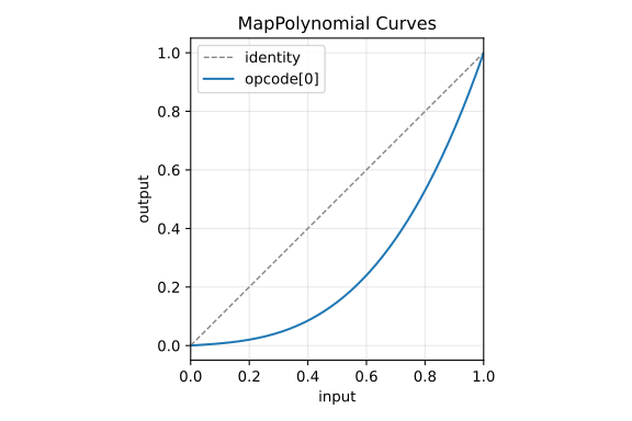
In short, it requires applying a polynomial mapping function to a specified region of the image. The LossyMosaicJXL mode uses a cubic polynomial, whose coefficients may be related to the maximum and minimum values of the RAW. It’s used to stretch the original RAW values, after black-and-white level correction, to a distribution that fills the entire 16-bit range.
This step actually increases the amount of data that needs to be compressed. If the original RAW is 14-bit and fills the value range, it adds (16 - 14) / 14 = 14.3% more data. The figure below shows the decoding function of the non-linear mapping for a RAW that fills the value range.
If the original RAW doesn’t fill the 14-bit range, then even more is added. An extreme example is a black-frame image, where the original RAW values might only be around 512 ± 20, yet after mapping they fill the entire 16-bit range, adding a huge amount of data. The figure below shows the decoding function of the non-linear mapping for a black-frame image.
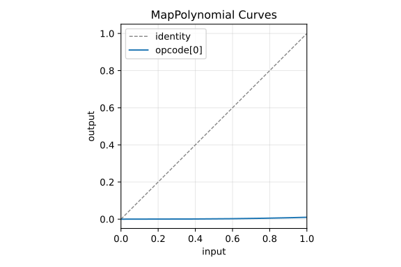
As a consequence, the file size of this black-frame image after stretching and then compressing with JPEG-XL reaches 20.8 MB, whereas encoding it directly with JPEG-XL’s lossless mode requires only 4.8 MB—a situation where the lossy mode is actually larger.
This non-linear mapping also serves the function of allocating more code values to the shadows, but this approach of directly stretching the values is currently debatable.
CFA RAW Rearrangement
When encoding a CFA RAW, the original image isn’t encoded directly. Instead, it’s rearranged according to the CFA layout, grouping pixels of the same colour together. This improves compression efficiency. The rearranged image is essentially several sub-images arranged together according to their original CFA positions.
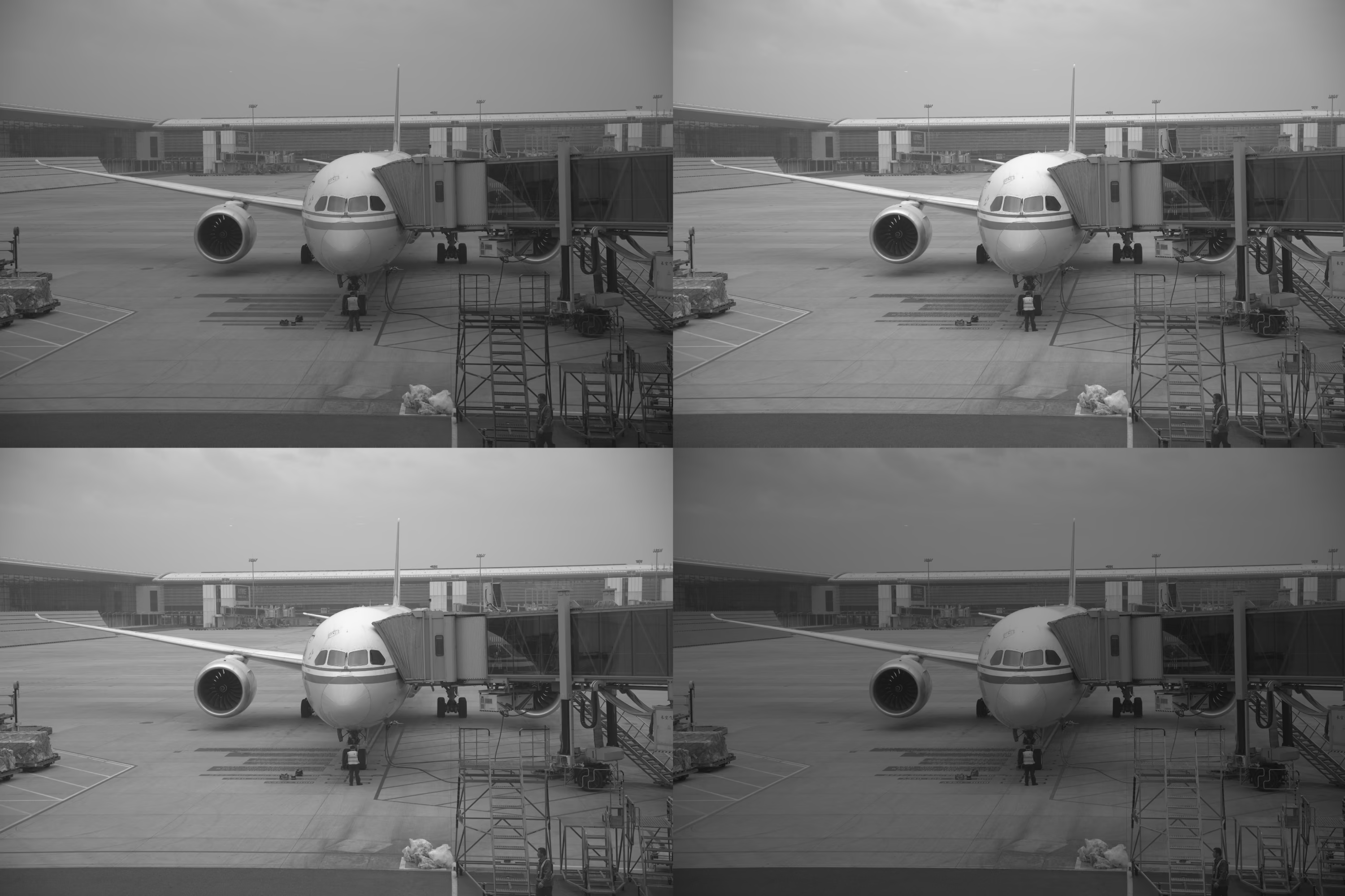
Taking that earlier RAW as an example again, the lossless-compressed JXL DNG produced by Adobe DNG Converter has a file size of 27.9 MB. Using the JXL encoder to encode the data in numpy array form directly in lossless mode as a simulation: if you encode the CFA RAW directly without rearrangement, the file size is 36.63 MB; after rearranging and then encoding, the file size is 26.77 MB, which is fairly close to Adobe’s result.
This advanced encoding format, JPEG-XL, also supports encoding multi-channel images. You can treat the different CFA positions as multiple channels, so the rearranged image is essentially a 4-channel image, and the file size obtained after encoding is 26.84 MB.
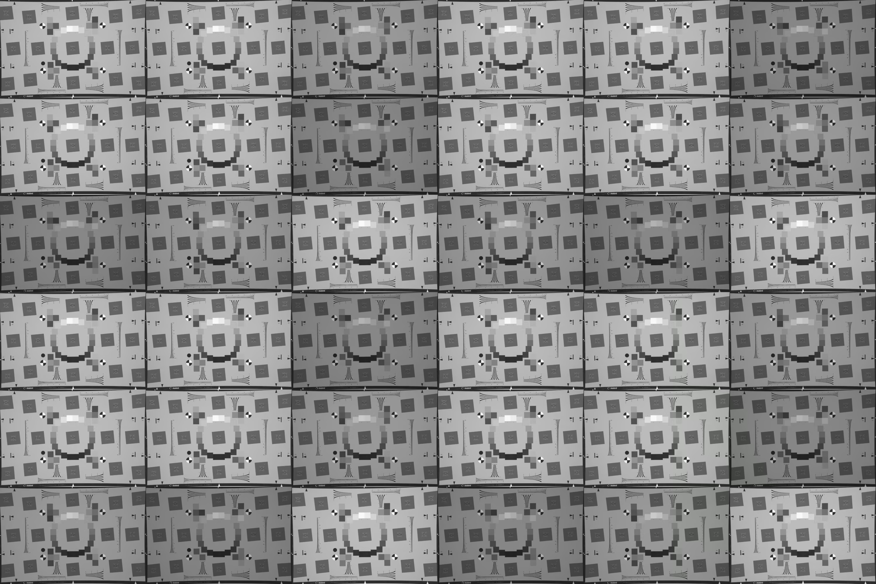
Fujifilm’s X-Trans, which has a more complex layout, works the same way—rearranged into X-Trans’s minimal repeating unit, which is 6x6, totalling 36 sub-images (looking at it gives me a bit of trypophobia).
What’s Next?
On the lossless front, a DNG encoded with JPEG-XL’s lossless mode is currently the best choice in terms of both compatibility and compression efficiency.
And for an image like RAW, which has relatively low information density, accepting a degree of lossy compression can dramatically improve compression efficiency. Currently, the two efficient lossy compression methods are DXO’s high-fidelity compression and Adobe DNG Converter’s LossyMosaicJXL mode, but both have some minor practical issues, such as whether it’s worth storing a 10-bit Linear RAW, and whether this non-linear mapping approach is reasonable.
Next, I’m going to experiment with some of JPEG-XL’s advanced settings, attempting to further improve compression efficiency while maintaining visual quality with only slight loss.